VAE 계열 모델의 ELBO(Evidence Lower Bound) 분석

RecVAE 모델을 분석하기 위해 논문을 읽으면서 VAE에 관해 모르거나 잘못 알고 있던 내용이 많다는 걸 알게 되어 이를 정리하고자 한다. 특히 ELBO 부분이 그전에는 잘 이해가 안 갔는데, 이번에 붙잡고 공부하면서 좀 더 명확히 이해할 수 있게 되었다. 그리고 VAE의 ELBO 유도 과정을 완전히 잘못 알고 있어서 복습하면서 정정했다.

 

 

VAE(Varational AutoEncoder) 한번에 이해하기

 

 

위의 노트 필기의 흐름을 따라가보면 VAE의 ELBO가 왜 loss function에서 나오는 건지와 그 학습 방법을 이해할 수 있다.

 

 

 

VAE 계열 모델의 ELBO 분석

VAE(Variational Autoencoders)

 

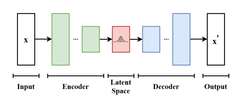
[출처] https://commons.wikimedia.org/wiki/File:VAE_Basic.png, EugenioTL

 

VAE(Variational Autoencoder)는 데이터를 Encoder에 넣어서 input보다 차원이 작은 latent space에서의 확률 분포에 관한 모수를 구하고, 이 latent space에서 앞서 구한 확률 분포로 샘플링하여 Decoder에 통해 새로운 이미지를 reconstruction 하는 비지도학습 모델이다. 이에 관한 자세한 내용은 이전 포스팅에서 다룬 바 있다.

 

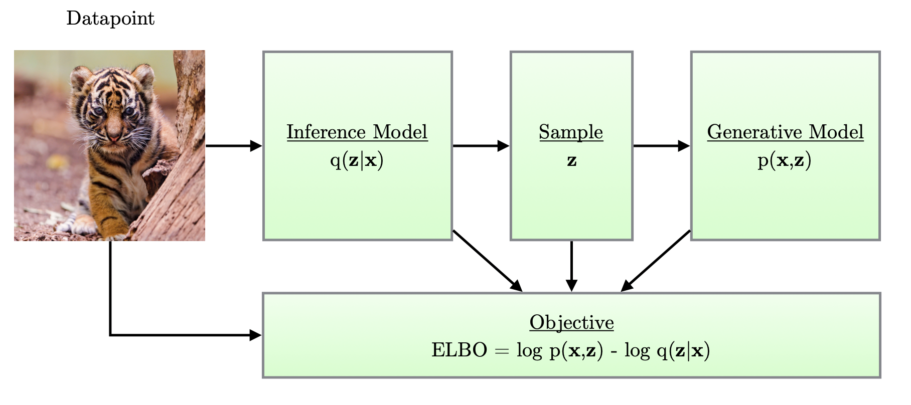
[출처] https://arxiv.org/pdf/1802.05814.pdf, Variational Autoencoders for Collaborative Filtering

 

https://glanceyes.tistory.com/entry/Deep-Learning-Generative-Model

생성 모델(Generative Model)과 VAE, 그리고 GAN

 

종종 VAE에서는 marginal likelihood function을 latent variable인 $z$로 나타낸다고 하는 얘기가 나오는데, 여기서 marginal likelihood function이 어떤 의미인지 모르겠어서 찾아보다가 이해에 도움이 되는 글을 찾았다.

 

https://m.blog.naver.com/sw4r/221380395720

[수리통계학] Marginal Likelihood 란? (빈도주의VS. 베이지안 관점 비교)

 

정리하자면, 베이즈 이론에서 Evidence에 해당되는 $x$에 대한 확률을 의미한다고 볼 수 있다.

 

들어가기에 앞서 우리는 VAE를 사용하고자 하는 목적부터 생각해봐야 한다.

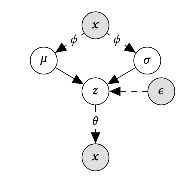
우리는 VAE에서 사후 확률 분포(posterior distribution)인 $p_{\theta }(z|x)$를 알고 싶은데 이를 직접 구하는 것은 어려우므로 이에 근사할 수 있는 사후 확률 분포(variational approximation of the posterior distribution)인 $q_{\varphi }(z|x)$를 찾는 변분 추론을 해야 한다.

우리의 최종 목적은 $q_{\varphi }(z|x)$와 $p_{\theta }(z|x)$ 분포의 차이를 줄이는 것임을 명심해야 하며, 이는 두 확률 분포의 KL Divergence인 $D_{KL}(q_{\varphi }(z|x)||p_{\theta }(z|x))$가 작아져야 됨을 뜻한다.

 

 

 

ELBO(Evidence Lower Bound)

이를 위해 marginal likelihood function인 $p_{\theta }(x)$를 나타내는 식을 정리하여 도출하는데, 이는 다음과 같다.

 

$$\begin{array}{rl}{p}_{\theta }(\mathbf{x})& ={\mathbb{E}}_{q_{\varphi }(z|x)}[\log p_{\theta }(x)]\\ & ={\mathbb{E}}_{q_{\varphi }(z|x)}[\log \frac{p_{\theta }(x,z)}{p_{\theta }(z|x)}]\\ & ={\mathbb{E}}_{q_{\varphi }(z|x)}[\log \frac{p_{\theta }(x,z)q_{\varphi }(z|x)}{q_{\varphi }(z|x)p_{\theta }(z|x)}]\\ & ={\mathbb{E}}_{q_{\varphi }(z|x)}[\log \frac{p_{\theta }(x,z)}{q_{\varphi }(z|x)}]+{\mathbb{E}}_{q_{\varphi }(z|x)}[\log \frac{q_{\varphi }(z|x)}{p_{\theta }(z|x)}]\\ & =\underset{\text{ELBO }\uparrow }{\underbrace{{\mathbb{E}}_{q_{\varphi }(z|x)}[\log \frac{p_{\theta }(x,z)}{q_{\varphi }(z|x)}]}}+\underset{\text{Objective }\downarrow }{\underbrace{D_{KL}(q_{\varphi }(z|x)||p_{\theta }(z|x))}}\end{array}$$

 

우리의 최종 목적을 달성하려면 뒤에 있는 항이 줄어들어야 하는 것이고, 이는 앞에 있는 ELBO(Evidence Lower Bound)를 증가시키면 된다.

사족이지만 처음에는 ELBO에서 왜 Evidence가 앞에 붙는지 이해를 못 했는데, marginal likelihood function이 결국 Evidence와 연관이 있다는 사실을 뒤늦게 깨달았다.

앞에 있는 ELBO를 정리하면 다음과 같다.

 

$$\begin{array}{rl}{\mathbb{E}}_{q_{\varphi }(z|x)}[\log \frac{p_{\theta }(x,z)}{q_{\varphi }(z|x)}]& =\int \ln \frac{p_{\theta }(x|z)p(z)}{q_{\varphi }(z|x)}{q}_{\varphi }(z|x)dz\\ & =\underset{\text{Reconstruction term}}{\underbrace{{\mathbb{E}}_{q_{\varphi }(z|x)}[\log p_{\theta }(x|z)]}}-\underset{\text{Prior Fitting Term}}{\underbrace{D_{KL}(q_{\varphi }(z|x)\Vert p(z))}}\end{array}$$

 

결국 ELBO는 두 개의 항으로 유도가 가능한데, 이는 Reconstruction Term과 Prior Fitting Term이다.

Reconstruction term은 encoder를 통해서 input을 latent space로 보내고 다시 decoder로 돌아오는 reconstruction loss을 줄이는 역할을 한다.

Latent space는 input 대상을 잘 설명할 수 있는 공간이며, input의 feature 중 일부는 다른 feature의 조합으로 표현 가능해서 불필요할 수 있으므로 latent space는 일반적으로 실제 space보다 작다.

Prior fitting term은 input을 latent space로 올렸을 때 이루는 latent distribution이자 앞에서 정한 근사 사후 확률 분포(variational approximation of the posterior distribution)를 prior distribution과 유사하도록 강화해주는 것이며, KL Divergence를 활용한다.

 

 

Amortized Inference

위에서 구한 ELBO와 marginal likelihood의 관계를 파악하여 논문에서 정리한 식에 맞게 정리하면 다음과 같다.

 

$$\begin{array}{r}\log p_{\theta }(x)\ge {\mathcal{L}}_{\text{VAE}}\\ & ={\mathbb{E}}_{q_{\varphi }(z|x)}[\log p_{\theta }(x|z)-\text{KL}(q_{\varphi }(z|x)\Vert p(z))]\end{array}$$

 

요약하면, 앞서 정리한 내용을 토대로 marginal likelihood는 최소한 ELBO보다는 크거나 같다는 것을 뜻한다.

 

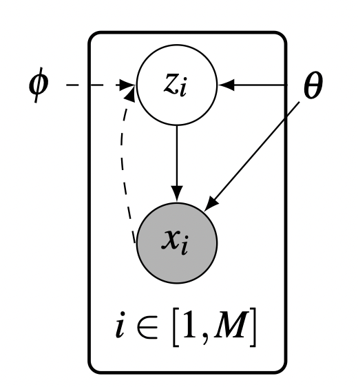
이러한 테크닉을 Amortized Inference라고 하며, 이를 통해 추가적인 정규화를 할 수 있고 variational parameters를 close form function으로 구할 수 있다. 또한 Encoder의 input인 서로 다른 $x_i$마다 다른 latent variable인 $z_i$를 만들어 내서 결과적으로 새로운 데이터가 들어올 때마다 발생하는 비용 문제를 효율적으로 해결할 수 있다고 한다.

 

[출처] https://arxiv.org/pdf/1711.05597.pdf, Advances in Variational Inference

 

Amortized Inference에 관해 잘 정리된 글이 있어서 이를 참조했다.

https://ricoshin.tistory.com/3

Amortized Inference란?

 

 

 

$\beta$-VAE(Beta-Variational Autoencoder)

VAE는 생성 모델이기도 하지만 representation을 학습할 수 있기도 하다. $\beta$-VAE는 VAE를 수정한 것이며, ELBO의 KL Divergence에 해당되는 Prior Fitting Term에 정규화 계수를 곱한 것이며, 이를 통해 disentangled represeation을 학습할 수 있다고 한다.

$\beta$-VAE의 목적 함수를 정리하면 다음과 같다.

 

$${\mathcal{L}}_{\beta -\text{VAE}}={\mathbb{E}}_{q_{\varphi }(z|x)}[\log p_{\theta }(x|z)-\beta \text{KL}(q_{\varphi }(z|x)\Vert p(z))]$$

 

 

DVAE(Denoising Variational Autoencoders)

DVAE(Denoising Variational Autoencoders)는 DAE(Denoising Autoencoders)와 유사하게 input에 noise를 추가하여 재건될 수 있도록 하는 모델이며, 이때의 ELBO는 다음과 같이 정의할 수 있다.

 

$$\begin{array}{r}\log p_{\theta }(x)\ge {\mathcal{L}}_{\text{DVAE}}\\ & ={\mathbb{E}}_{q_{\varphi }(z|\tilde{x})}{\mathbb{E}}_{p(\tilde{x}|x)}[\log p_{\theta }(x|z)-\text{KL}(q_{\varphi }(z|\tilde{x})\Vert p(z))]\end{array}$$

 

여기서는 VAE와 달리 input인 $x$에 확률적으로 noise를 주기 위해 ${\mathbb{E}}_{p(\tilde{x}|x)}$가 추가되었다. 이 $p(\tilde{x}|x)$는 일반적으로 베르누이 분포나 가우시안 분포로 설정한다. DAE에서와 마찬가지로 DVAE에서도 input에 noise를 추가함으로써 기존 VAE보다 좀 더 강건하고 더 나은 일반화 성능을 보인다.

 

이에 관한 자세한 내용은 아래 논문을 통해서 볼 수 있다.

https://arxiv.org/abs/1511.06406

Denoising Criterion for Variational Auto-Encoding Framework

 

 

CVAE(Conditional Variational Autoencoder)

CVAE(Conditional Variational Autoencoder)는 좀 더 복잡한 조건부 확률을 학습하기 위해 구현한 VAE의 연장선으로 볼 수 있다. ELBO 식을 정의하면 다음과 같다.

 

$$\begin{array}{rl}\log p_{\theta }(x|y)& \ge {\mathcal{L}}_{\text{CVAE}}=\\ & {\mathbb{E}}_{q_{\varphi }(z|x,y)}[\log p_{\theta }(x|z,y)-\text{KL}(q_{\varphi }(z|x,y)\Vert p(z,y))]\end{array}$$

 

모든 확률 분포가 $y$라는 확률 변수에 의해 조정된다는 것을 알 수 있다.

 

 

VAEAC(VAE with Arbitrary Conditioning)

 

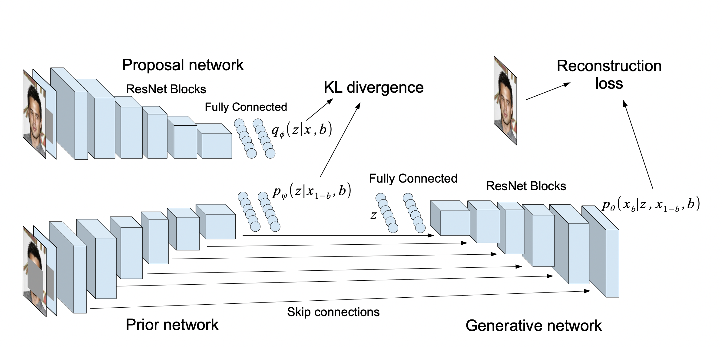
[출처] https://arxiv.org/pdf/1806.02382.pdf, Variational Autoencoder with Arbitrary Conditioning

 

VAEAC(VAE with Arbitrary Conditioning)는 여기서 더 나아가 missing feature를 위한 imputation problem을 해결하기 위해 제안되었으며, 많은 부분에 있어서 Collaborative Filtering과 비슷하다.

 

VAEAC의 ELBO는 Binary mask인 $b$에 관하여 CVAE의 ELBO에서 변수에 대응되는 건 관측되지 않은 feature를 의미하는 $x_b$로, 조건에 대응되는 건 $x_{1-b}$로 나타낸 것과 같다.

 

$$\begin{array}{rl}\log p_{\theta ,b}(x_b|x_{1-b},b)& \ge {\mathcal{L}}_{\text{VAEAC}}=\\ & {\mathbb{E}}_{q_{\varphi }(z|x,b)}[\log p_{\theta }(x_b|z,x_{1-b},b)-\text{KL}(q_{\varphi }(z|x,b)\Vert p(z|x_{1-b},b))]\end{array}$$

 

중요한 점은 mask $b$는 서로 다른 input $x$에 관해 모두 다를 수 있고, 관측되지 않은 feature를 뜻하는 마스크의 1의 개수도 다를 수 있다. 하지만 이러한 접근법은 직접 바로 implicit feedback에 적용할 수는 없다고 한다.

 

 

업데이트
1. 'VAE 한번에 이해하기' 항목을 추가하고 노트필기 이미지를 첨부했습니다. (2023. 03. 19)
2. 'VAE 한번에 이해하기' 항목의 잘못된 내용을 수정했습니다. (2023. 05. 23)